A while back we discussed what systematic correction is and how the files are created to apply this to your data. As a follow up, today we’ll explain how the content of systematic correction files are used.

Systematic correction creates a parametric model (Linear, Quadratic) based on the GC fractions of the probe sequence and its neighborhood. The parameters are estimated by the least-square method, minimizing the sum of squares of the difference between the data and the modeled value. The model value is calculated by plugging in the estimated parameters and then subtracted from the original probe value to get the corrected value.

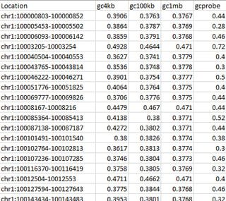
For example, take the correction file values as shown below:

Location gc4kb gc100kb gc1mb gcprobe
chr1:1301-1351 0.3825 0.3780 0.3767 0.4615
chr1:1350-1399 0.3731 0.3781 0.3769 0.4625
…

and the log2 ratio for probes in these regions:
chr1:1324-1325 0.3
chr1:1374-1375 0.4

…

Then a linear model is created:
0.3 = a*0.3825 + b*0.3780 + c*0.3767 + d*0.4615 + e
0.4 = a*0.3731 + b*0.3781 + c*0.3769 + d*0.4625 + e

…

and solved for the parameters a,b,c,d and e with the least-squares method
and results in a=0.001,b=0.0001,c=0.00001,d=0.3, e=-0.1

These parameters are multiplied to get the estimated GC bias values:
0.001*0.3825 + 0.0001*0.3780 + 0.00001*0.3767 + 0.3*0.4615 – 0.1 = 0.0388
0.001*0.3731 + 0.0001*0.3781 + 0.00001*0.3769 + 0.3*0.4625 – 0.1 = 0.0391

The GC bias for probes in these two regions are subtracted from the original to get the corrected probe values:
chr1:1324-1325 0.3-0.0388 = 0.2612
chr1:1374-1375 0.4-0.0391 = 0.3609